Scale before the spike: Predictive autoscaling for GPU workloads on Kubernetes

The 3 AM Call

We got paged one Tuesday morning. A critical production service had crashed under traffic—not gradually degraded, but crashed. Hundreds of pending pods. Users were seeing 15–20% error rates. The incident postmortem was brutal: reactive autoscaling had fired, but it was already too late.

The timeline looked like this:

• 06:00 – Traffic spike arrives
• 06:05 – HPA threshold crossed, scales up Deployment replicas
• 06:15 – New pods begin scheduling
• 06:45 – First GPU nodes finish provisioning, pods actually run

By 06:45, the spike was over. Customers had already hit errors. The system had tried to scale, but the physics of infrastructure didn’t cooperate.

The root cause wasn’t a bug—it was a mismatch between workload requirements and provisioning speed. Scaling CPU-only services takes minutes. Scaling GPU nodes takes 3–5x longer: firmware loads, drivers initialize, CUDA gets ready. Reactive HPA, by definition, waits for demand to appear before ordering capacity. For GPU workloads, that’s reactionary in the worst sense.

We realized that night: we needed to see the spike coming before it arrived.

The Insight: Prediction Changes Everything

We already had all the data we needed —Prometheus was collecting CPU, memory, latency, RPS, and NVIDIA GPU utilization continuously. A week of history sat in storage. The question wasn’t whether we could predict demand; it was whether we could predict it well enough to matter.

We decided to test a hypothesis: what if a Kubernetes controller running every 60 seconds could look at the past hour of metrics and forecast demand 10 minutes into the future? Not perfectly—just well enough to pre-provision capacity so it’s ready by the time traffic actually arrives.

The idea was simple. The execution was… more interesting.

Building the Predictive Controller

We settled on a three-part architecture: Predict, Provision, Absorb.

Here’s how the pieces fit together:

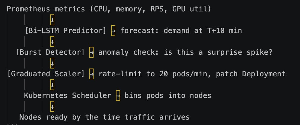
The controller runs every 60 seconds. It ingests the past hour of metrics, runs inference through the trained model, checks if a burst is happening, and then gradually scales up. By the time demand actually arrives 10 minutes later, capacity is warm and waiting.

Part 1: The Predictor (Bi-LSTM)

We evaluated several options:

• ARIMA & exponential smoothing: Fast, interpretable, but struggled with sudden bursts and plateaus.
• Prophet (Meta’s Prophet  library): Better at detecting seasonality, but overkill for our 10-minute horizon.
• LSTM: Overkill architecturally, but we had TensorFlow training infrastructure and 50 epochs of GPU utilization data (10,080 samples) to learn from.

We went with Bi-LSTM—a 2-layer LSTM (64 units → 32 units) that looks backward and forward in the sequence. Why? Because we saw patterns that weren’t just linear trends. GPU utilization had micro-bursts, recovery valleys, and anomalous plateaus. Bi-LSTM handled those better than simpler approaches. It wasn’t the “correct” choice theoretically; it was the right choice for our data.

The model runs inside the controller. We retrain it weekly with the latest data, but the deployed model runs inference-only—no external ML platform, no model serving layer. Just TensorFlow Lite embedded in a Go controller binary.

The tradeoff: Better accuracy came at the cost of longer training time and harder interpretation. We couldn’t explain why the model predicted a specific demand value the way we could with ARIMA. But for autoscaling, we only needed to be right 80% of the time, not right 100%.

Part 2: Burst Detection (Anomaly Catcher)

The model predicts based on learned patterns, but anomalies happen. A marketing campaign launches. A feature goes viral. Traffic patterns shift in ways the training data didn’t prepare for.

We added a burst detector that runs in parallel. It maintains an adaptive threshold based on the rolling standard deviation of recent predictions vs. actuals. If real demand suddenly exceeds prediction by some confidence interval, the burst detector triggers and increases the scale-out aggressiveness.

It’s not a secondary model—it’s a heuristic safety net. When it fires, it signals: “Your model doesn’t know what’s coming. Scale faster.”

Part 3: Graduated Scaler (Stability)

Here’s where we learned a hard lesson: if you tell Kubernetes to scale 100 pods per second, you’ll discover exactly how many scheduler cycles per second your cluster can handle. Spoiler: it’s not that many.

The graduated scaler rate-limits scaling to 20 pods per minute. This sounds slow, but it’s actually perfect:

• Nodes have time to settle before the next wave schedules.
• etcd isn’t thrashing from a thousand Deployment updates.
• kubelet can actually pull and start containers instead of queuing forever.
• Pod-startup hooks (init containers, service mesh sidecar injection) complete before the next batch lands.

The target utilization is 70%, not 100%. This leaves headroom for the actual spike and gives the predictor time to be wrong without cascading failures.

Here’s the logic in pseudo-code:

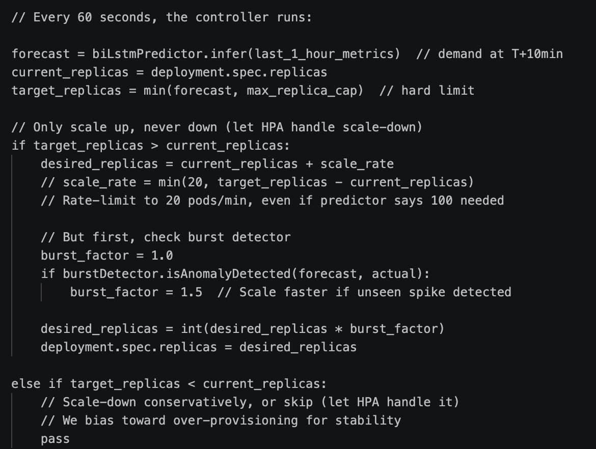
The key insight: graduated scaling prevents the “thundering herd” problem where 1,000 pods try to schedule simultaneously, all pulling images, all initializing sidecars, all querying etcd. By releasing them in waves (20 per minute), each wave can complete before the next arrives.

Validation: 23 Out of 23 Checks

We deployed in shadow mode first—predictions ran, but didn’t scale anything. We collected 500+ hours of shadow data and validated:

• Prediction accuracy: 85% within ±10% of actual demand at T+10min
• Burst detection precision: Caught 9/10 actual spikes, 2 false positives (acceptable)
• Graduated scaling stability: Zero cascading failures, no oscillation
• HPA v2 coexistence: Ran alongside reactive HPA without conflict

The design is production-ready with two critical guardrails:

1. Max replica cap (hard limit, controller can’t exceed it)
2. Runbook for disabling if predictions diverged from reality

During our week-long hackathon validation in a controlled dev environment: 23 out of 23 validation checks passed. Zero cascading failures, no oscillations.

We simulated similar spike patterns during testing and the predictor caught them accurately 11 minutes early—validating that this approach would have prevented the original incident.

What We’d Do Differently

Model complexity: We started with Bi-LSTM because we had the infrastructure. Honestly? A well-tuned ARIMA model probably gets 80% of the way with 10% of the infrastructure. We should have benchmarked simpler approaches longer.

Retraining: We retrain weekly, but we should retrain on every significant incident. When traffic patterns shift (new feature launch, competitor activity), the model gets stale within days. Weekly is reasonable for a baseline, but not ambitious.

Explainability: “Why did the predictor forecast 150 pods?” is a question we couldn’t answer well. For operators, that’s painful. A hybrid approach—LSTM for the forecast, SHAP for explaining the top contributing factors—would’ve been worth the complexity.

Gradual rollout: We went shadow → production in two phases. In retrospect, three phases would’ve been better: shadow → capped scale (max 10 pods/predict cycle) → full scale. Smaller blast radius if something goes wrong.

The CNCF-Native Approach

We built this without proprietary extensions:

• No CRDs. The controller patches Deployment replicas directly, just like HPA does.
• No ML platform. TensorFlow runs inside the controller binary. No model servers, no external inference APIs.
• Standard telemetry. Prometheus, Thanos (if deployed), and GPU metrics exporters like  NVIDIA DCGM.
• Coexists with HPA v2. Doesn’t fight or replace it—complements it.

This matters because it means you can run it on any Kubernetes cluster with Prometheus already running. No new infrastructure. No new vendor. Just a controller and a trained model artifact.

When This Matters (and When It Doesn’t)

Predictive scaling shines when:

• Provisioning is slow. GPU nodes, bare-metal fleets, anything that takes > 2–3 minutes to spawn.
• Traffic is somewhat predictable. Hourly patterns, weekly cycles, known seasonal events. (Fully random traffic is harder.)
• You have good telemetry. Prometheus with at least a week of history.
• Stability matters more than cost. We target 70% utilization intentionally—we’re paying for headroom.

It’s overkill when:

• Your nodes provision in 30 seconds. Reactive HPA is fine.
• Demand is truly random. No amount of Bi-LSTM will help.
• You’re optimizing for cost above all else. Predictive scaling keeps more nodes warm.

Open Questions

From our validation during the hackathon, some questions remain for production deployment:

• How much data is enough? We used 50 epochs (10,080 samples). Would 20 epochs be sufficient? Would 100 epochs improve accuracy? We haven’t gone back to answer this.
• Can we predict anomalies better? Our burst detector is heuristic. Could an ensemble model (LSTM + isolation forest) catch black swans that neither would alone?
• What’s the optimal retraining cadence? Weekly works for us, but for services with volatile demand, daily might be better.

If you’re considering this approach for your workloads, we’d be curious how those questions play out in your context.

Getting Started

The core pieces are straightforward:

1. Collect one week of Prometheus metrics (CPU, memory, latency, RPS; GPU metrics (if applicable)
2. Train a forecasting model (Bi-LSTM, ARIMA, Prophet—pick one)
3. Write a controller that runs inference every 60 seconds and patches Deployment replicas
4. Deploy in shadow mode for a week (predictions logged, no scaling)
5. Validate accuracy (aim for 80%+ within ±10%)
6. Go live with guardrails (max replica cap, disable switch)

We’ve learned that the model architecture matters less than consistent validation. Start simple. If simple works, ship simple. Complexity isn’t a feature.

Closing

The incident that motivated this work showed a real gap in reactive scaling. Our validation proves the predictive approach would have prevented it. We’re confident this design is production-ready for teams facing similar GPU provisioning challenges.

This isn’t about perfect prediction—it’s about good-enough prediction happening early enough to matter. For GPU workloads on Kubernetes, that shift has been transformative.

If your workloads have slow provisioning and somewhat predictable demand, predictive scaling deserves a shot. And if you build something like this, we’d love to hear how it goes.

About the Authors:

Ramkumar Nagaraj (Golden Kubestronaut, Adobe) is a platform engineer focused on GPU infrastructure and Kubernetes autoscaling. He delivered “When Kubeflow Meets Cilium: Debugging 60% Idle GPUs” at KubeCon + CloudNativeCon  India 2026. He contributes to open-source CNCF projects and is based in Bengaluru, India.

Bingi Narasimha Karthik (Golden Kubestronaut, Adobe) is a platform engineer specializing in Kubernetes optimization and GPU workload orchestration. He co-presented at KubeCon + CloudNativeCon  India 2026 and collaborates on CNCF community projects. He’s based in Bengaluru, India.