


Guest post by Marcelo Amaral, Sunyanan Choochotkaew, Eun Kyung Lee, Huamin Chen, and Tamar Eilam
Stepping into the exciting world of technology where things are always on the move, we’re introduced to cool new applications like the ones powered by generative AI (using ChatGPT, Google Bard, and IBM WatsonX APIs). But, have you ever wondered what’s happening in the background? Data centers are putting in a lot of work that accounts for hundreds metric tons of CO2 each year [1].
In the current tech landscape, it’s not just about what we can do with technology, but also about how much energy, CO2 and cost we’re consuming. Governments are pushing for more efficient energy consumption to minimize the impact on the environment. This is why there’s a strong focus on measuring energy use and finding ways to save power. Even cloud providers are getting in on the action by sharing monthly reports on how much carbon footprint their customers are creating.
But here’s the big question: How much energy do these applications that live in the cloud really use? Can we get even more detailed and measure it down to the second? The answer is a definite yes. The Kepler project steps in, letting us measure how much power applications consume. Of course, there are challenges and limitations to consider in different situations. In this blog post, we’re diving deep into the Kepler architecture, exploring different scenarios. Stick around to get a closer look at how this powerful tool works behind the scenes on Bare-metal or Virtual Machines.
Kepler Architecture
Kepler, Kubernetes-based Efficient Power Level Exporter, offers a way to estimate power consumption at the process, container, and Kubernetes pod levels. The architecture is designed to be extensible, enabling industrial and research projects to contribute novel power models for diverse system architectures.
In more details, Kepler utilizes a BPF program integrated into the kernel’s pathway to extract process-related resource utilization metrics. Kepler also collects real-time power consumption metrics from the node components using various APIs, such as Intel Running Average Power Limit (RAPL) for CPU and DRAM power, NVIDIA Management Library (NVML) for GPU power, Advanced Configuration and Power Interface (ACPI) for platform power, i.e, the entire node power, Redfish/Intelligent Power Management Interface (IPMI) also for platform power, or Regression-based Trained Power Models when no real-time power metrics are available in the system.
Once all the data that is related to energy consumption and resource utilization are collected, Kepler can calculate the energy consumed by each process. This is done by dividing the power used by a given resource based on the ratio of the process and system resource utilization. We will detail this model later on in this blog. Then, with the power consumption of the processes, Kepler aggregates the power into containers and Kubernetes Pods levels. The data collected and estimated for the container are then stored by Prometheus.
Kepler finds which container a process belongs to by using the Process ID (PID) information collected in the BPF program, and then using the container ID, we can correlate it to the pods’ name. More specifically, the container ID comes from /proc/PID/cgroup, and Kepler uses the Kubernetes APIServer to keep an updated list of pods that are created and removed from the node. The Process IDs that do not correlate with a Kubernetes container are classified as “system processes” (including PID 0). In the future, processes that run VMs will be associated with VM IDs so that Kepler can also export VM metrics.
Cloud infrastructures, like Kubernetes where most cloud applications commonly run, offer deployment options either through Bare-metal (BMs) environments or Virtual Machines (VMs) on public clouds. The choice depends on the desired level of control for the customer.
When it comes to measuring energy consumption, there’s a notable distinction between Bare-metal and VMs on public clouds. Bare metal nodes provide power metrics directly from their hardware components, such as the CPU and DRAM. For instance, in x86 machines using RAPL, or ACPI. In contrast, VMs do not expose power metrics. The primary reason behind this is the absence of mechanisms to make these metrics available (Kepler could help cloud providers in the future!). This divergence leads Kepler to employ a different approach for these two distinct scenarios, which we will explain next.
Collecting System Power Consumption – VMs versus BMs
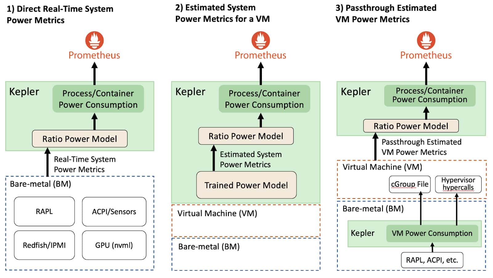
Depending on the environment that Kepler was deployed in, the system power consumption metrics collection will vary. For example, consider the figure above, Kepler can be deployed either through BMs or VMs environments.
In bare-metal environments that allow the direct collection of real-time system power metrics, Kepler can split the power consumption of a given system resource using the Ratio Power model. But before explaining the Ratio Power model, we first need to introduce some concept related to the power metrics. The APIs that expose the real-time power metrics export the absolute power, which is the sum of the dynamic and idle power. To be more specific, the dynamic power is directly related to the resource utilization and the idle power is the constant power that does not vary regardless if the system is at rest or with load. This concept is important because the idle and dynamic power are splitted differently across all processes. Now we can describe the Ratio Power model, which divides the dynamic power across all processes.
The Ratio Power model calculates the ratio of a process’s resource utilization to the entire system’s resource utilization and then multiplying this ratio by the dynamic power consumption of a resource. This allows us to accurately estimate power usage based on actual resource utilization, ensuring that if, for instance, a program utilizes 10% of the CPU, it consumes 10% of the total CPU power. The idle power estimation follows the GreenHouse Gas (GHG) protocol guideline [2], which defines that the constant host idle power should be splitted among processes/containers based on their size (relative to the total size of other containers running on the host). Additionally, it’s important to note that different resource utilizations are estimated differently in Kepler. We utilize hardware counters to assess resource utilization in bare-metal environments, using CPU instructions to estimate CPU utilization, collecting cache misses for memory utilization, and assessing Streaming Multiprocessor (SM) utilization for GPUs utilization.
In VM environments on public clouds, there is currently no direct way to measure the power that a VM consumes. Therefore, we need to estimate the power using a trained power model, which has some limitations that impact the model accuracy, which we further detail later in this blog. However, there is another approach that Kepler could help cloud providers to expose the VM power metrics, enabling accurate estimation of the workload power consumption within the VMs. In this approach, Kepler is first deployed in the bare-metal node (i.e., the cloud control plane), and it continuously measures the dynamic and idle power that each VM consumes using real-time power metrics from the BM. Then, Kepler exposes this power data with the VM. This information can be made available to the VM through “hypervisor Hypercalls” [3] or by saving the numbers in special files that the VM can access (e.g., cGroup file mounted in the VM). Then, by using the VM power consumption, another Kepler instance within the VM can apply the Ratio Power Model to estimate the power used by processes residing in the VMs.
Nonetheless, while the passthrough approach is still not available, Kepler can estimate the dynamic power consumption of VMs using trained power models. Then, after estimating each VM’s power consumption, Kepler applies the Ratio Power Model to estimate the processes’ power consumption. However, since VMs usually do not provide hardware counters, Kepler uses eBPF metrics instead of hardware counters to calculate the ratios. It is important to highlight that trained power models used for VMs on a public cloud cannot split the idle power of a resource because we cannot know how many other VMs are running in the host. We provide more details in the limitation section in this blog. Therefore, Kepler does not expose the idle power of a container running on top of a VM.
Power models are trained by performing regression analysis (like Linear or Machine Learning (ML)-based regression) on data collected during benchmark tests. This data includes both resource utilization and power consumption on a Bare-metal node, forming the foundation for the power model estimation. We’ll dive into the details of training these power models next.
Model Server Power Model Training
The Model Server is used to train power models, and it can be optionally deployed alongside Kepler to help Kepler select the most appropriate power model for a given environment. For example, considering the CPU model, available metrics and the required model accuracy. In the future, Kepler will also be able to select the power model with the same logic that the Model Server has.
The Model Server trains its models using Prometheus metrics from a specific bare-metal node. It records how much energy the node consumed and the resource utilization of containers and system processes (OS and other background processes). The container metrics are obtained from running various small tests that stress different resources (CPU, memory, cache, etc.), like using a tool called stress-ng. When creating the power model, the Model Server uses a regression algorithm. It keeps training the model until it reaches an acceptable level of accuracy. Once trained, the Model Server makes these models accessible through a github repository, where any Kepler deployment can download the model from. Kepler then uses these models to calculate how much power a node (VM) consumes based on the way its resources are being used. The type of metrics used to build the model can differ based on the system’s environment. For example, it might use hardware counters, or metrics from tools like eBPF or cGroups, depending on what is available in the system that will use the model.
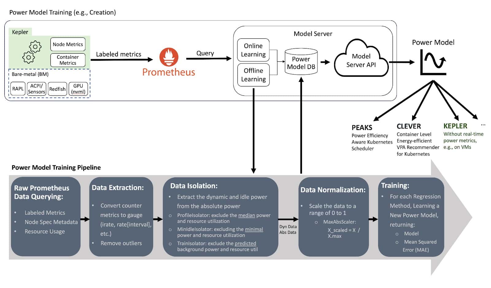
Let’s now dive deeper into the pipeline process of training power models in the Model Server. The figure above illustrates the steps involved in creating these models. It all starts with collecting data from Prometheus through various queries. This data includes power-related metrics from the node, with source labels specifying components like RAPL and platform power from ACPI, as well as node specifications like CPU model and architecture. Additionally, it collects metrics related to resource utilization by the node, containers and OS/System background processes. After data collection, the next step is data extraction. The data extraction involves converting counter metrics to gauge metrics with per second values using similar Prometheus functions irate and rate, where those functions can smooth the data depending on the defined interval. We call this dataset as absolute data since it includes both the dynamic and idle power and the aggregated resource utilization of all processes.
Following the gauge metric extraction, the dynamic power is isolated from the absolute data for training purposes. Therefore, models created after the data isolation are called dynamic power models (DynPower). Note that models created without this data isolation are referred to as absolute power models (AbsPower), which estimates absolute power: idle + dynamic power. The advantage of using a dynamic power model is the better accuracy to estimate the dynamic power.
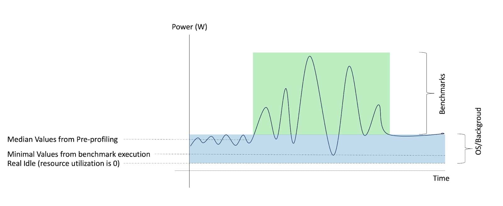
Before running the benchmarks, the system is in a state where only the OS and background process are running, although there might be some other user workloads running concurrently. During data collection, we capture power and resource utilization information both before and during the execution of the benchmark tests, as illustrated in the Figure above. After that, to isolate the dynamic power associated with the benchmark tests, we can employ three distinct techniques:
- ProfileIsolator: This isolator uses initial samples collected before the benchmark tests, referred as pre-profiling. It calculates the median power and resource utilization values during this phase. These pre-profiling values are then subtracted from the absolute values of the dataset to extract the dynamic power specific to the benchmarks.
- MinIdleIsolator: This isolator extracts the minimum values observed during the benchmark experiments from the absolute values of the dataset. However, it’s worth noting that the extracted values may include some data from the operating system and background processes in the training, as it captures the lowest values across all measurements, but these other processes also have dynamic utilization.
- TrainIsolator [4]: The TrainIsolator takes a different approach. It initially trains a power model using the absolute values of the dataset, including both idle and dynamic power data. This trained model is then used to estimate the actual idle power (when resource utilization is at zero) and the power consumed by the operating system and background processes. These estimated values are subtracted from the overall dataset, leaving only the power and resource utilization data directly associated with the benchmark tests. This ensures that the dynamic power component is isolated for training purposes.
Note that our isolators are an ongoing project, and we anticipate making improvements and expansions in the future. One potential future enhancement is the inclusion of an isolator described in the IEEE Cloud WIP paper [5], which also accounts for the activation power.
After the data isolation, before training the power model, the data is normalized because different metrics are on different scales. A simple normalization can be dividing the metrics by the max value. Lastly, the processed data is used to train models with multiple regression algorithms, and the model with the lowest mean squared error is selected to be used. The created power model can be used not only by Kepler when running in a system that does not have real-time power metrics, but also by other tools such as Power Efficiency Aware Kubernetes Scheduler (PEAKS) [6], or Container Level Energy-efficient VPA Recommender for Kubernetes (CLEVER) [7]. These tools leverage the power model to make informed decisions about power consumption and resource allocation in a more energy-efficient manner. Finally, the created power models can be shared publicly through GitHub repository [8].
Pre-trained Power Model Limitations
It’s important to note that pre-trained power models have their limitations when compared to power models using real-time power metrics.
Firstly, pre-trained power models are specific to the system architecture. Different CPU models and architectures exhibit unique power consumption patterns [9], as illustrated in the figure below for Intel Xeon Platinum 8260, Intel Xeon E5-2697 v4 and E5-2667 v3 (each of these machines have 2 sockets). This means that different power models are needed for different systems. Nevertheless, even though a generic power model does not reflect 100% of the physical host, it can provide some insight into the application power consumption, helping optimization tools make better overall energy-efficient decisions.
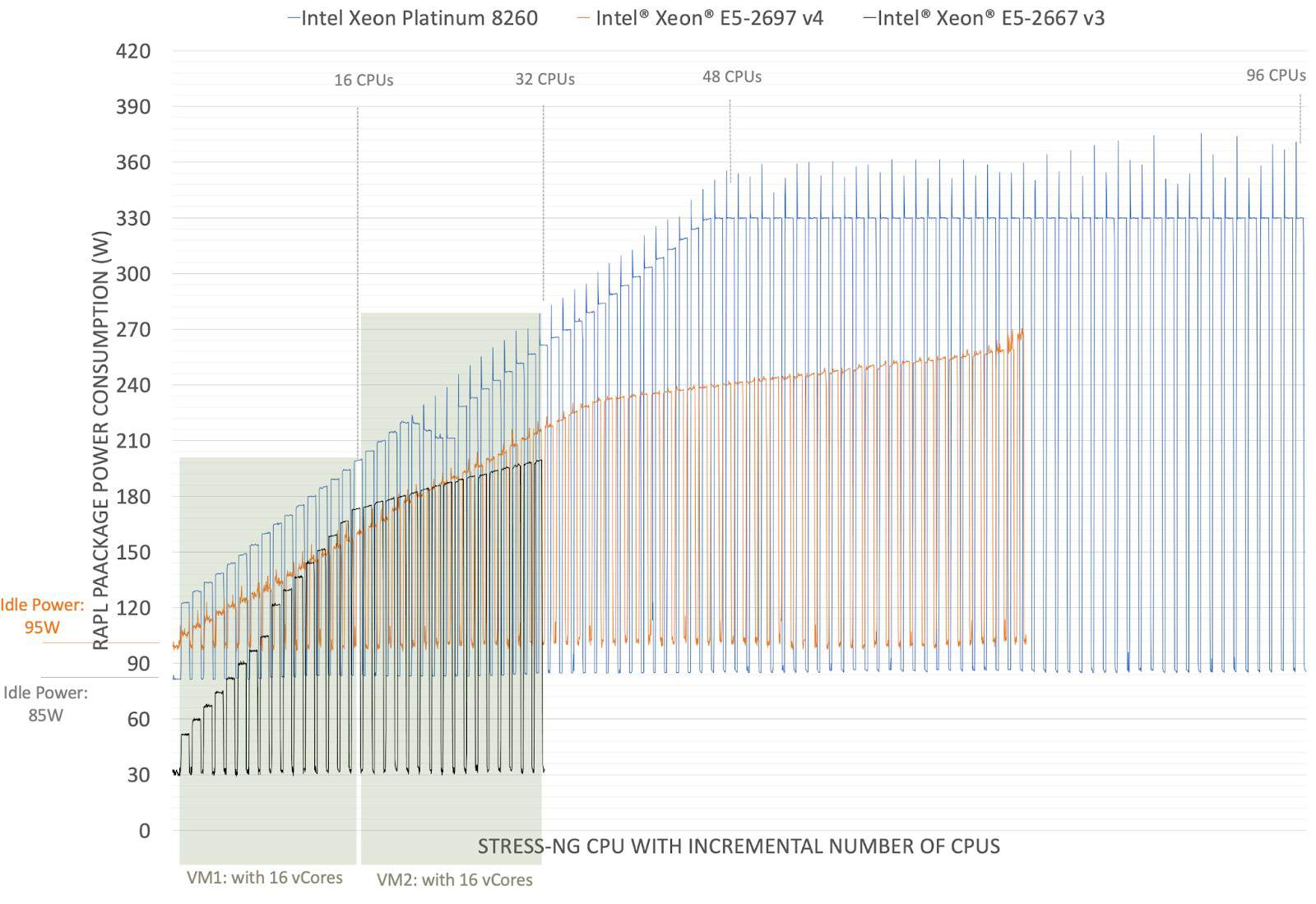
Secondly, using the bare-metal power model for single VMs can lead to overestimation of the power. In a typical scenario in a public cloud, a bare-metal node might host multiple VMs, where each VM represents a fraction of the total node resource utilization. The problem here is that the VMs running on the node will estimate power consumption based on the initial part of the BM power curve. For example, as illustrated in the figure above, consider a VM with 16 virtual CPUs (vCores) running on a node with an Intel Xeon Platinum 8260. According to the power model, this VM will consume 110W of dynamic power (205W of absolute power – 95W of idle power) when all its CPUs are working at full speed (e.g., running stress-ng cpu workload). Now, if we apply this power model to two VMs, each with 16 vCores, both fully using the CPUs, they would report that each of them are using 110W, which is in total 220W. However, the BM power curve shows us something different. It shows that the machine actually uses less power when more CPUs are in use. So, when these two VMs together use 32 CPUs, they consume up to 180W, not 220W.
This problem can be even more complicated because power models can have a plateau, which means a point where they don’t use much more power even if you add more workload. In the case of the Intel Xeon Platinum 8260, this plateau is at around 350 watts with 48 CPUs (note that the node has 48 physical CPUs with 2 hyper-threads). Now, let’s say there are six VMs, each with 16 vCores (for a total of 96 vCPUs). The real power consumption would be maximum of 370W due to the plateau, but if each VM uses its power model individually, they might mistakenly report a total power consumption of around 660W (6 * 110W). Therefore, without knowing the total resource utilization of the host, it is very hard to estimate the total host power consumption and the aggregated VM power consumption will be overestimated.
Thirdly, there is the issue of idle power since according to the GHG protocol, the constant host idle power should be splitted among VMs based on their size (relative to the total size of other VMs running on the host). However, within a VM on a public cloud, determining the number of concurrently running VMs on the host is not currently possible. This makes it difficult to appropriately divide the idle power. Note that we cannot just use the host idle power without splitting it between all running VMs since each running VM would otherwise duplicate the host idle power giving the wrong idea about how much idle power each VM and the host actually uses. As a result, pre-trained power models for VMs can only estimate the dynamic power consumption. As dynamic power is directly related to resource utilization, Kepler’s power model can effectively estimate VM dynamic power.
Fourthly, it’s important to highlight that Kepler pre-trained power models for VMs rely on the hypervisor’s accurate reporting of CPU register values. This dependency is crucial for Kepler’s calculations, assuming that the resources allocated to VMs on the node are appropriately managed and not oversubscribed. However some VMs in public cloud have their resource overprovisioned, which will impact the accuracy of the resource utilization metrics collected within the VM.
Work in Progress Challenges
The Kepler community is diligently working on adding exciting and useful functionalities and improving the performance of the kepler. The currently working in progress challengers are as follows:
- Extra Data Import Support: One of the key focuses of the Kepler community is to broaden its horizons by providing extra power data import support, e.g., power source from Board Management Controller (BMC), IPMI support [10], and RedFish support [11], for power estimation/model. Kepler is gearing up to handle additional data power sources with greater accuracy to estimate the energy, making it more versatile and adaptable to user’s needs.
- Vendor and Architecture-Agnostic Kepler Support: Another addition is its support for various vendors/hardware architectures. This means you won’t be tied to specific HW vendors when using Kepler (e.g., CPU, GPU, server vendors). This is to ensure the user can gain the energy estimation regardless of the architecture/hardware vendor the user uses. This support will make Kepler more versatile and inclusive in the community.
- Performance Boost by understanding Overhead: The Kepler community is also dedicated to boost its performance of Kepler. To enhance performance, Kepler is undergoing a meticulous overhead analysis. The overhead analysis involves examining every aspect of the Kepler and the system to identify and address bottlenecks, e.g., kepler-exporter scraping frequency, eBPF sampling frequency, Prometheus data import overhead, and node/pod scalability. By understanding where the system may be slowing down or experiencing inefficiencies, Kepler can be optimized for a smoother and more responsive user experience.
- Overhead Remediation: The Kepler community is also actively working on overhead remediation approaches. This includes innovative solutions like adaptive and adjustable sampling techniques, as well as delay compensation approaches. These strategies will help Kepler report the system/platform energy, ensuring that the user gets real-time insights on energy consumption without any performance hiccups.
- Multi level Kepler Deployment: To tackle the challenge of accurately estimating the power of each virtual machine (VM), we can use Kepler with a multi-level deployment approach. In this approach, Kepler is first deployed in the bare-metal node (i.e., the cloud control plane), and it continuously measures the dynamic and idle power that each VM consumes using real-time power metrics from the BM. Then, Kepler shares this power data with the VM. This information can be made available to the VM through “hypervisor Hypercalls” or by saving the numbers in special files that the VM can access (e.g., cGroup file). Now, inside the VM, a second-level Kepler can use this exposed power information to estimate how much power the containers within the VM are using. We hope that with the growing demand from industry and governments of accurate power metrics, the public cloud would leverage Kepler to expose VM power metrics.
Try it out
Get VMs or BMs on IBM Cloud or AWS Cloud to create a Kubernetes cluster, or create an OpenShift Cluster, where you can deploy Kepler. Check out also:
Reference
- Data Centres and Data Transmission Networks, https://www.iea.org/energy-system/buildings/data-centres-and-data-transmission-networks
- ICT Sector Guidance built on the GHG Protocol Product Life Cycle Accounting and Reporting Standard. 2017. https://www.gesi.org/research/ict-sector-guidance-built-on-the-ghg-protocol-product-life-cycle-accounting-and-reporting-standard
- KVM Hypercalls. https://docs.kernel.org/virt/kvm/x86/hypercalls.html
- Advancing Cloud Sustainability: A Versatile Framework for Container Power Model Training. IEEE MASCOTS Workshop 2023. (in press)
- Kepler: A framework to calculate the energy consumption of containerized applications. IEEE CLOUD WIP 2023. https://research.ibm.com/publications/kepler-a-framework-to-calculate-the-energy-consumption-of-containerized-applications
- PEAKS github. https://github.com/sustainable-computing-io/peaks
- CLEVER github. https://github.com/sustainable-computing-io/clever
- Kepler github. https://github.com/sustainable-computing-io/kepler
- Intel Xeon W Review. https://www.anandtech.com/show/13116/the-intel-xeon-w-review-w-2195-w-2155-w-2123-w-2104-and-w-2102-tested/2
- IPMI document: https://www.ibm.com/docs/en/power9/0009-ESS?topic=ipmi-overview
- Redfish document: https://www.dmtf.org/standards/redfish