
Guest post originally published on Pixie’s blog by Omid Azizi and Pete Stevenson
Application profiling tools are not new, but they are often a hassle to use. Many profilers require you to recompile your application or at the very least to rerun it, making them less than ideal for the lazy developer who would like to debug performance issues on the fly.
Earlier this year, we built the tool we’d like to have in our personal perf toolkit – a continuous profiler that is incredibly easy to use: no instrumentation, no redeployment, no enablement; just automatic access to CPU profiles whenever needed.
Over the next 3 blog posts, we’ll show how to build and productionize this continuous profiler for Go and other compiled languages (C/C++, Rust) with very low overhead (<1% and decreasing):
- Part 1: An intro to application performance profiling.
- Part 2: A simple eBPF-based CPU profiler.
- Part 3: The challenges of building a continuous CPU profiler in production.
Want to try out Pixie’s profiler before seeing how we built it? Check out the tutorial.
Part 1: An Introduction to Application Performance Profiling
The job of an application performance profiler is to figure out where your code is spending its time. This information can help developers resolve performance issues and optimize their applications.
For the profiler, this typically means collecting stack traces to understand which functions are most frequently executing. The goal is to output something like the following:
70% main(); compute(); matrix_multiply()10% main(); read_data(); read_file() 5% main(); compute(); matrix_multiply(); prepare()...
Above is an example stack traces from a profiler. Percentages show the number of times a stack trace has been recorded with respect to the total number of recorded stack traces.
This example shows several stack traces, and immediately tells us our code is in the body of matrix_multiply() 70% of the time. There’s also an additional 5% of time spent in the prepare() function called by matrix_multiply(). Based on this example, we should likely focus on optimizing matrix_multiply(), because that’s where our code is spending the majority of its time.
While this simple example is easy to follow, when there are deep stacks with lots of branching, it may be difficult to understand the full picture and identify performance bottlenecks. To help interpret the profiler output, the flamegraph, popularized by Brendan Gregg, is a useful visualization tool.
In a flamegraph, the x-axis represents time, and the y-axis shows successive levels of the call stack. One can think of the bottom-most bar as the “entire pie”, and as you move up, you can see how the total time is spent throughout the different functions of your code. For example, in the flamegraph below, we can see our application spends 80% of its time in compute(), which in turn spends the majority of its time in matrix_multiply().
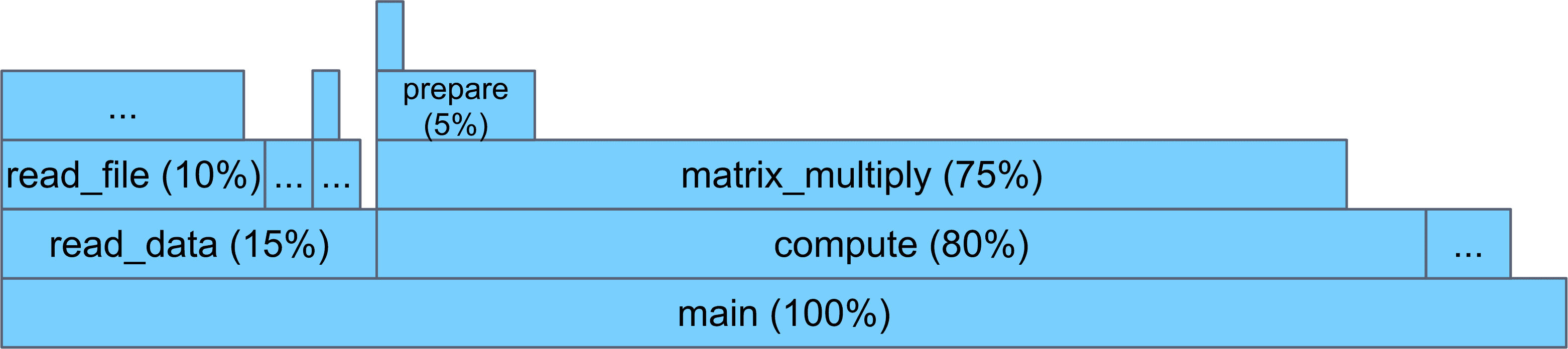
In a flamegraph, wide bars indicate program regions that consume a large fraction of program time (i.e. hot spots), and these are the most obvious candidates for optimization. Flamegraphs also help find hot spots that might otherwise be missed in a text format. For example, read_data() appears in many sampled stack traces, but never as the leaf. By putting all the stack traces together into a flamegraph, we can immediately see that it consumes 15% of the total application time.
How Do Profilers Work Anyway?
So profilers can grab stack traces, and we can visualize the results in flamegraphs. Great! But you’re probably now wondering: how do profilers get the stack trace information?
Early profilers used instrumentation. By adding measurement code into the binary, instrumenting profilers collect information every time a function is entered or exited. An example of this type of profiler is the historically popular gprof tool (gprof is actually a hybrid profiler which uses sampling and instrumentation together). Unfortunately, the instrumentation part can add significant overhead, up to 260% in some cases.
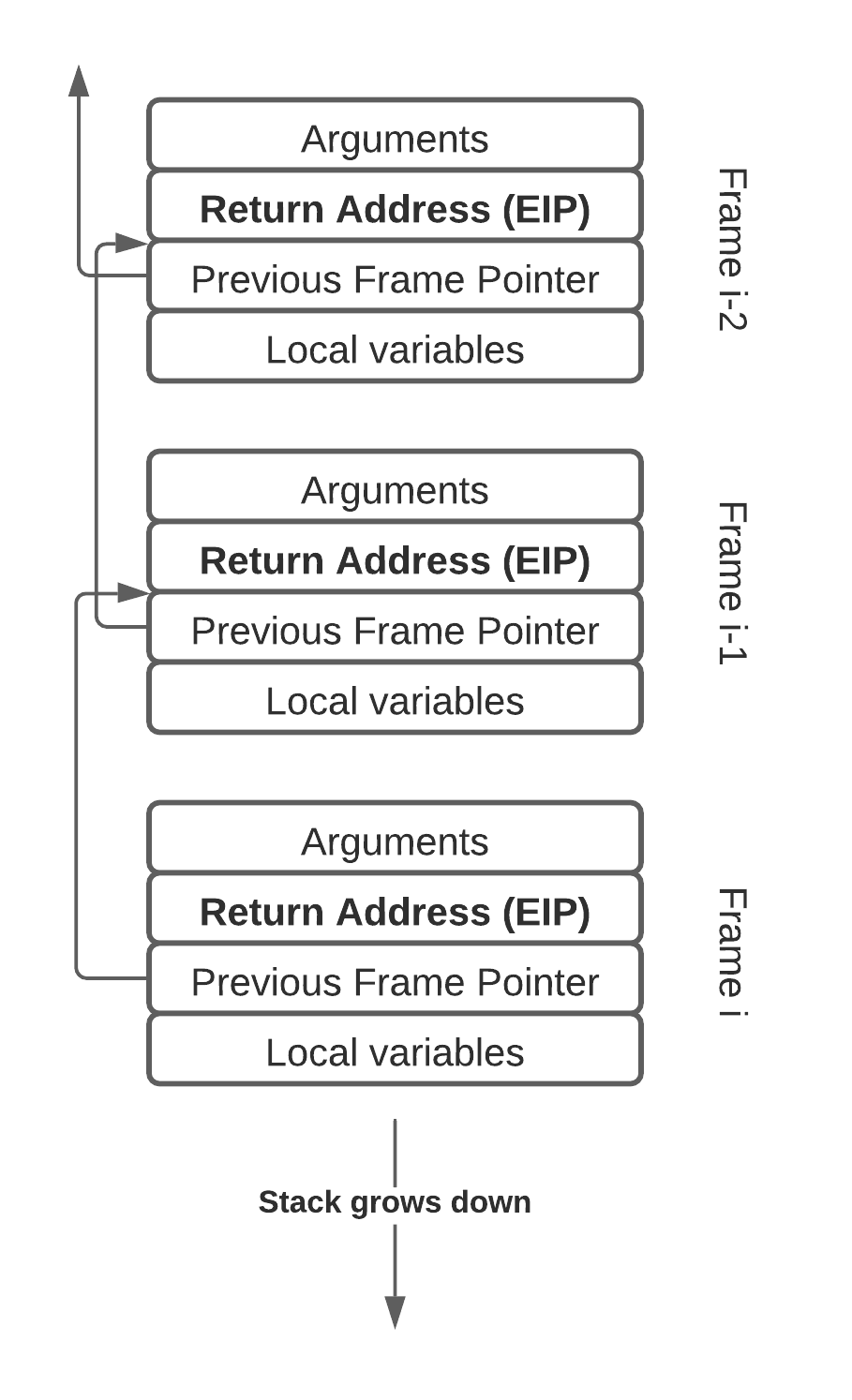
More recently, sampling-based profilers have become widely used due to their low overhead. The basic idea behind sampling-based profilers is to periodically interrupt the program and record the current stack trace. The stack trace is recovered by looking at the instruction pointer of the application on the CPU, and then inspecting the stack to find the instruction pointers of all the parent functions (frames) as well. Walking the stack to reconstruct a stack trace has some complexities, but the basic case is shown below. One starts at the leaf frame, and uses frame pointers to successively find the next parent frame. Each stack frame contains a return address instruction pointer which is recorded to construct the entire stack trace.
By sampling stack traces many thousands of times, one gets a good idea of where the code spends its time. This is fundamentally a statistical approach, so the more samples are collected, the more confidence you’ll have that you’ve found a real hot-spot. You also have to ensure there’s no correlation between your sampling methodology and the target application, so you can trust the results, but a simple timer-based approach typically works well.
Sampling profilers can be very efficient, to the point that there is negligible overhead. For example, if one samples a stack trace every 10 ms, and we assume (1) the sampling process requires 10,000 instructions (this is a generous amount according to our measurements), and (2) that the CPU processes 1 billion instructions per second, then a rough calculation (10000*100/1B) shows a theoretical performance overhead of only 0.1%.
A third approach to profiling is simulation, as used by Valgrind/Callgrind. Valgrind uses no instrumentation, but runs your program through a virtual machine which profiles the execution. This approach provides a lot of information, but is also high in overheads.
The table below summarizes properties of a number of popular performance profilers.
| Profiler | Methodology | Deployment | Traces Libraries/System Calls? | Performance Overhead |
|---|---|---|---|---|
| gprof | Instrumentation + Sampling | Recompile & Rerun | No | High (up to 260%) |
| Callgrind | Simulation | Rerun | Yes | Very High (>400%) |
| gperftools | Sampling (User-space only) | Rerun | Yes | Low |
| oprofile, linux perf, bcc_profile | Sampling (Kernel-assisted) | Profile any running process | Yes | Low |
For Pixie, we wanted a profiling methodology that (1) had very low overheads, and (2) required no recompilation or redeployment. This meant we were clearly looking at sampling-based profilers.
In part two of this series, we’ll examine how to build a simple sampling-based profiler using eBPF and BCC.